Meter Readings Over MQTT

In a previous post I talked about swapping the in-home device (IHD) supplied by my electricity and gas company for one produced by Glow. This connects over wifi and gives access to the raw data coming from your smart meters over MQTT. To collect this data and integrate it into my house monitor I needed to listen to the MQTT topic and expose the data to Prometheus.

This was quite similar to my previous project to expose statistics from my router, but as this was processing JSON data being exposed over MQTT it was a lot simpler than parsing raw text over SSH. As before I created a GitHub repo with my usual Python linting, testing and build scripts set up.

Connecting to MQTT is straightforward, using the Paho MQTT library. When they’ve set up your MQTT account Glow’s support team will supply you with a topic name that you can use, along with the username and password you set, to connect. The code below shows how to do this. We’ll cover the on_message callback next.

def connect(args, on_message):
    client = mqtt.Client()
    client.on_connect = functools.partial(on_connect, args.topic)
    client.on_message = on_message

    client.username_pw_set(args.user, password=args.passwd)
    client.connect("glowmqtt.energyhive.com", 1883, 60)

    client.loop_forever()

As you can probably guess, the on_message callback is called every time you receive a message on your MQTT topic. In our case, this will be the raw ZigBee data encoded as a JSON object. This GIST has a good summary of the available values, so I won’t repeat them here. The details for the electricity meter are included under elecMtr then 0702. There are a series of values for daily, weekly and monthly usage, but the most useful is the raw meter reading. We can extract this like so:

elec_multiplier = int(elecMtr["03"]["01"], 16)
elec_divisor = float(int(elecMtr["03"]["02"], 16))
elec_meter = int(elecMtr["00"]["00"], 16)

electricity_meter = elec_meter * elec_multiplier / elec_divisor

The raw meter reading sent a hex-encoded integer, which is scaled by the given multiplier and divisor. Why it’s like that I’m not sure, but I do appreciate Glow providing as low-level data as they can, even if it requires us to deal with some oddities like this. Once you’ve decoded and scaled the meter reading we can expose the metrics to Prometheus in the usual way.

The queries I’m using in Grafana are as follows:

rate(meter{type="electricity"}[5m])*1000*3600

increase(meter{type="gas"}[30m])*10

The electricity query is multiplied by 1000 as the raw data is in kilowatts, and the graphs look better when Grafana converts from watts in kilowatts itself. rate returns the per second rate, but as the number we want is kilowatts per hour we multiply it by 3600. The gas query is simpler - as the data is sent only once per half hour we look at the increase in the last 30 minutes. The raw data appears to be in tens of cubic meters, so we multiply by 10 to get the right value.

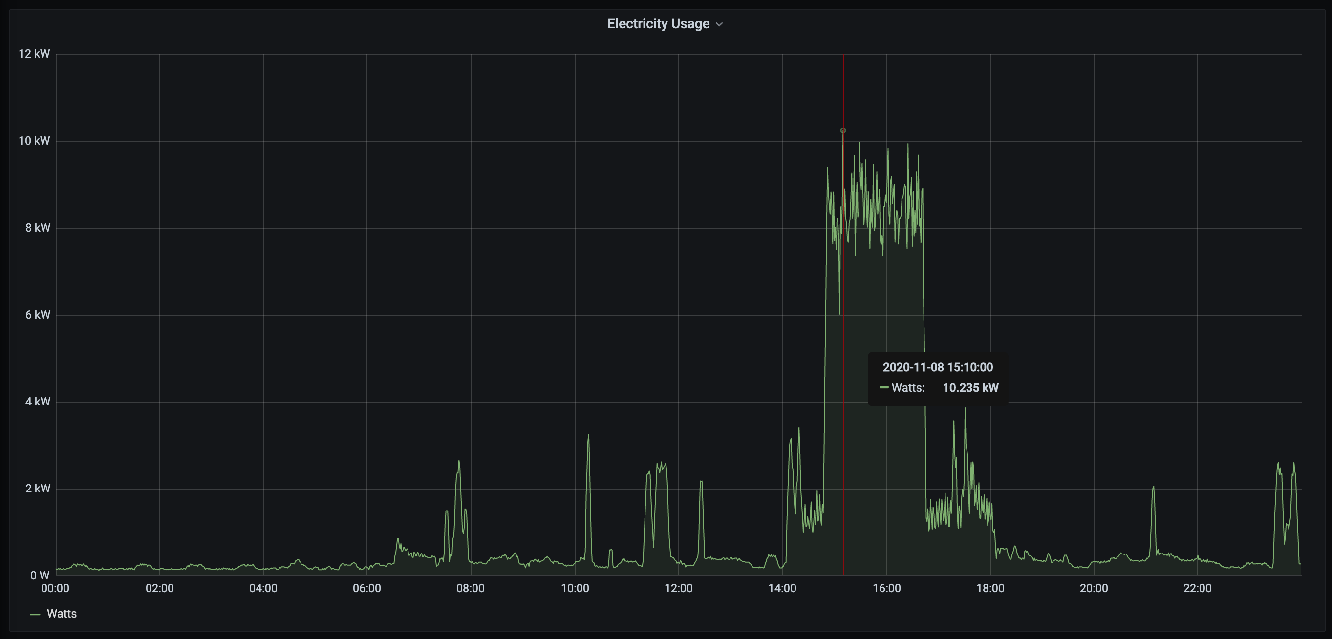
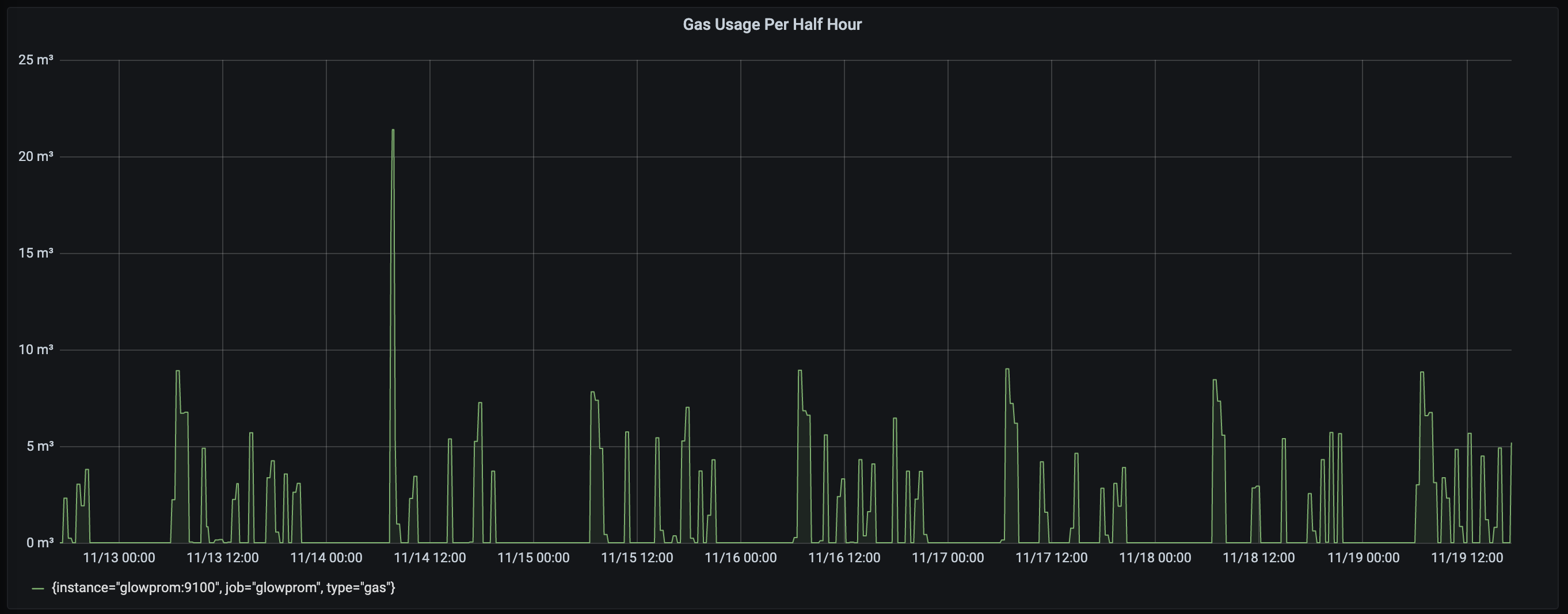
The graphs above show my usage electricity over the course of a day, and gas over a week. In the electricity graph, you can clearly see when the oven was on (2 pm-6 pm) and when I was charging my car (3 pm-5 pm). Other spikes during the day are the kettle or toaster being used. The peak right at the end is our dishwasher starting. Even in the middle of the night, our fridge running is clearly visible as a series of regular peaks. The gas data is much noisier, although you can see when we get up and go to bed. I think a longer analysis of gas usage will probably be more interesting.

Photo Electricity by Richard Graham.